
Linear regression is more than 200 years old algorithm is used for predicting properties with a training data set.
In this blog we will learn
Linear Regression
Simple linear regression is a straight line equation between independent and dependent variables. That straight equation is
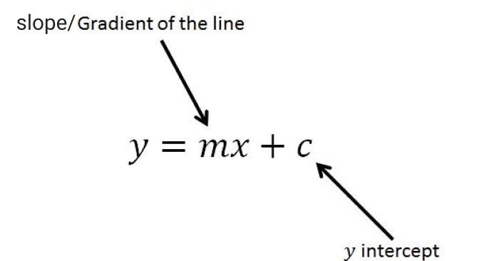
Here, y is a dependent variable on x (an independent variable). We will need to estimate slope and the y intercept from the training data set and once we get these coefficients we can use this equation any value for y given x as input. But why this straight line equation?
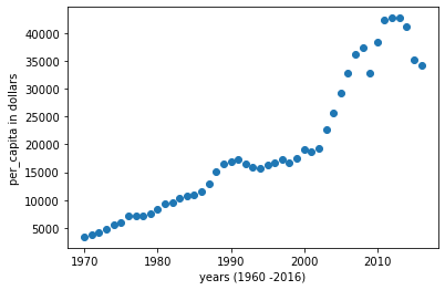
Suppose that we have this data for the per capita income of the US(in dollars) for the years 1970 to 2016.
I will represent the data using a jupyter notebook, and various python libraries such as pandas, numpy sklearn, matplotlib with an alias name.
|
import pandas as pd import numpy as np import matplotlib.pyplot as plt |
and plot the available data(training data set) using a scatter plot diagram.
The first five rows and the 2 columns of the data is as follows
|
df = pd.read_csv(‘percapita.csv’) df.head() # first five rows of the file |
|
year |
per_capita |
|
|
0 |
1970 |
3399.299037 |
|
1 |
1971 |
3768.297935 |
|
2 |
1972 |
4251.175484 |
|
3 |
1973 |
4804.463248 |
|
4 |
1974 |
5576.514583 |
Now plotting the above data with 46 columns and 2 rows
|
%inline matplotlib plt.scatter(df.year,df.per_capita) |
<matplotlib.collections.PathCollection at 0x7f3a4437e208>
Now there could be more than one line of equations which satisfies the condition for finding the regression or prediction values as.
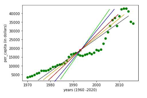
But to find the best line which fits the regression with the least error value we will need to calculate the coefficients of the equation.
So to calculate these coefficients, you’ll need to calculate the mean of both the properties first, and then find their difference from mean.
|
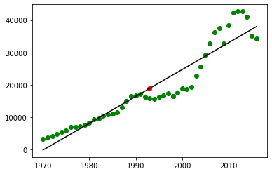
plt.xlabel(‘years (1960 -2016)’) plt.ylabel(‘per_capita in dollars’) plt.scatter(df.year,df.per_capita) plt.scatter(np.mean(df.year),np.mean(df.per_capita),color=’red’) |
<matplotlib.collections.PathCollection at 0x7f3d8322e898>
Now to draw a relation between these points we will need a straight line equation using Least Square Method (to have the least difference between predicted line and the observed values).
So these coefficients can be calculated with
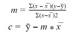
Here, (x – x̅ )is the difference between the actual points of x and the mean value(1993.0) and (y-ȳ)is the difference between the actual value of y from the mean point (18920.1370).
|
year |
per_capita_income(US$) |
x-x̅ |
y-ȳ |
(x-x̅)2 |
(y-ȳ)(x-x̅) |
|
1970 |
3399.299037 |
23 |
-15,520.837963 |
529 |
-3,56,979.273149 |
|
1971 |
3768.297935 |
22 |
-15,151.839065 |
484 |
-3,33,340.45943 |
When you have calculated slope(m),in this case {828.46507522} the equation for the mean value of x and y will be
18920.1370 = {828.46507522}*1993.0 + c
Which on further calculation will give,
c = -1632210.7578554575
So now the equation, for any point of value will be
y = {828.46507522}*x + {-1632210.7578554575}
And there you are to predict any value of per capita for a given year.
Check out this Online Data Science Course by Fita, which includes Supervised,Unsupervised machine learning algorithms,Data Analysis Manipulation and visualisation,reinforcement testing, hypothesis testing and much more to make an industry required data scientist at an affordable price, which includes certification, support with career guidance assistance.
Or with a python function it can be implemented as
|
#covariance between x and y def covar(x,x_mean,y,y_mean): covariance = 0.0 for i in range(len(y)): covariance += (x[i] – x_mean) * (y[i] – y_mean) return covar
#variance for difference between actual and mean value def variance(values): return np.var(values)
# slope and intercept def coefficients(row_1,row_2): x_mean, y_mean = np.mean(row_1), np.mean(row_2) slope = covar(row_1,x_mean,row_2,y_mean)/variance(row_1) intercept = x_mean – (slope * y_mean) return [slope, intercept]
def simple_linear_regression(df,test_values): predictions = [] m, x = coefficients(df[[‘years’]],df[[‘per_capita’]]) for i in test_values: y_values = x + m * i predictions.append(y_values) return predictions |
Estimate regression equation using sklearn
And now here’s how you would do it with python sklearn library.Import linear_model from the library and create an instance of it.
|
from sklearn import linear_model reg = linear_model.LinerRegression() |
|
# passing per capita as a dependent variable on per capita reg.fit(df[[‘years’]],df.per_capita) |
Now the model is ready for a best fit equation line, we can find out the slope and the y intercept with reg.coef_ and reg.intercept_
|
reg.coef_ reg.intercept_ |
Which outputs
|
828.46507522 -1632210.7578554575 |
Now let us visualise the data with matplotlib
|
plt.xlabel(‘years (1960 -2020)’) plt.ylabel(‘per_capita (in dollars)’) plt.scatter(np.mean(df.year),np.mean(df.per_capita),color=’red’) plt.plot(df.year,reg.predict(df[[‘year’]]),color=’black’) |
[<matplotlib.lines.Line2D at 0x7fa1daffbba8>]
and then use the predict method to predict any value of per capita for a given year.
|
reg.predict([[2020]]) |
Output
|
41288.69409442 |
Now let’s predict the per capita for recent years(testing data set) ,and store them in a csv file
|
df_2 = pd.read_csv(‘years.csv’) df_2.head() |
|
year |
|
|
0 |
2016 |
|
1 |
2017 |
|
2 |
2018 |
|
3 |
2019 |
|
4 |
2020 |
Now store the predicted values in the new column of the years.csv file.
|
predicts = reg.predict(df_2) df_2[‘predicted_per_capita’] = predicts # creating new column df_2.to_csv(‘predictions.csv’) # creating new file df_2.head() # first five rows of the file |
|
year |
predicted_per_Capita |
|
|
0 |
2016 |
37974.833794 |
|
1 |
2017 |
38803.298869 |
|
2 |
2018 |
39631.763944 |
|
3 |
2019 |
40460.229019 |
|
4 |
2020 |
41288.694094 |
You might notice the difference between the actual value of 2016 and the predicted value of 2016. This is known as mean squared error, and the correctness of the equation can be found with the R Square Method also known as coefficient of determination or coefficient of multiple determination. This R2can be calculated with the following formula.
R2=(yp-ȳ)(xp-x̅ )
If the more the R2is less than 1 the more the values are far the regression line.
This was all about linear regression algorithm with an example of predicting per capita income of US for several years with a trained data set.To get in-depth knowledge of Python along with its various applications and real-time projects, you can enroll in Python Training in Chennai or Python Training in Bangalore by FITA or enroll for a Data science course at Chennai or Data science course in Bangalore which includes Supervised, Unsupervised machine learning algorithms, Data Analysis Manipulation and visualisation, reinforcement testing, hypothesis testing and much more to make an industry required data scientist at an affordable price, which includes certification, support with career guidance assistance.
